Signals processing

Basis

In case I am not going to learn this field very comprehensively, this note would only contain the info.s that useful to my research.

Most of the notes are based on references gievn by Scipy.signal.

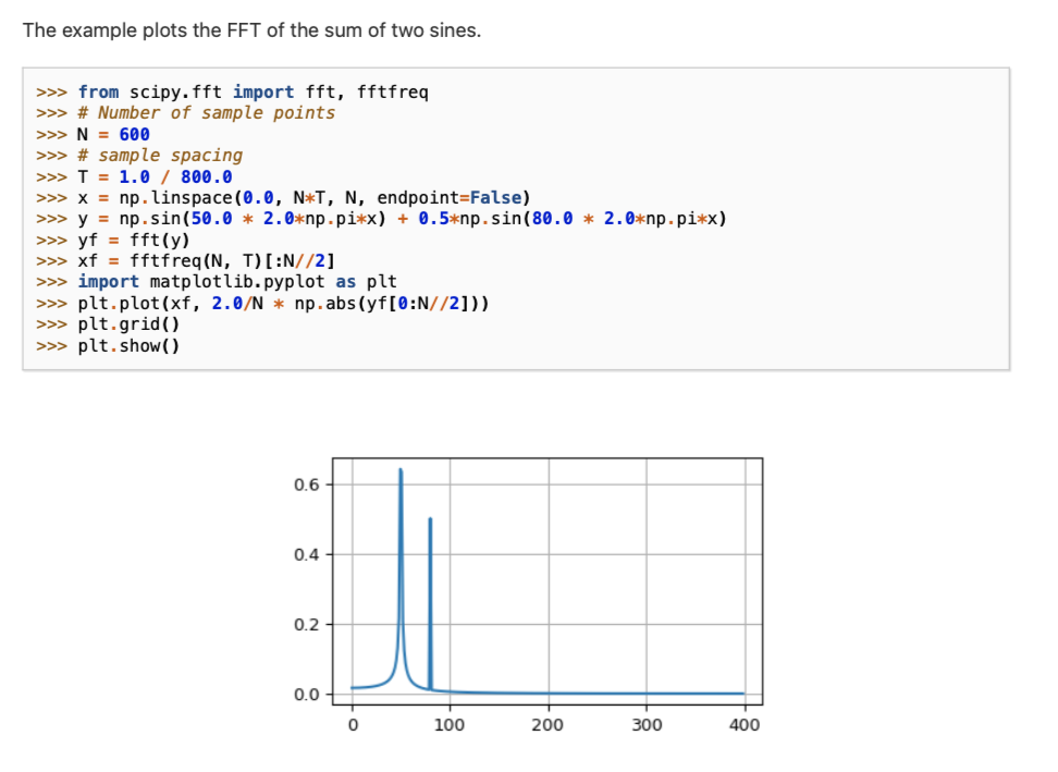
FFT

The FFT \(y[k]\) of length \(N\) of the length- \(N\) sequence \(x[n]\) is defined as \[ y[k]=\sum_{n=0}^{N-1} e^{-2 \pi j \frac{k n}{N}} x[n] \] and the inverse transform is defined as follows \[ x[n]=\frac{1}{N} \sum_{k=0}^{N-1} e^{2 \pi j \frac{k n}{N}} y[k] . \] These transforms can be calculated by means of fft and ifft, respectively, as shown in the following example.

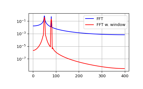
Window

The FFT input signal is inherently truncated. This truncation can be modeled as multiplication of an infinite signal with a rectangular window function. In the spectral domain this multiplication becomes convolution of the signal spectrum with the window function spectrum, being of form \(\sin(x)/x\). This convolution is the cause of an effect called spectral leakage (see [WPW]). Windowing the signal with a dedicated window function helps mitigate spectral leakage. The example below uses a Blackman window from scipy.signal and shows the effect of windowing (the zero component of the FFT has been truncated for illustrative purposes).

from scipy.fft import fft, fftfreq
import numpy as np
>>> # Number of sample points
>>> N = 600
>>> # sample spacing
>>> T = 1.0 / 800.0
>>> x = np.linspace(0.0, N*T, N, endpoint=False)
>>> y = np.sin(50.0 * 2.0*np.pi*x) + 0.5*np.sin(80.0 * 2.0*np.pi*x)
>>> yf = fft(y)
>>> from scipy.signal import blackman
>>> w = blackman(N)
>>> ywf = fft(y*w)
>>> xf = fftfreq(N, T)[:N//2]
>>> import matplotlib.pyplot as plt
>>> plt.semilogy(xf[1:N//2], 2.0/N * np.abs(yf[1:N//2]), '-b')
>>> plt.semilogy(xf[1:N//2], 2.0/N * np.abs(ywf[1:N//2]), '-r')
>>> plt.legend(['FFT', 'FFT w. window'])
>>> plt.grid()
>>> plt.show()

Spectral leakage

频谱泄漏（spectral leakage）: 信号为无限长序列，运算需要截取其中一部分（截断），于是需要加窗函数，加了窗函数相当于时域相乘，于是相当于频域卷积，于是频谱中除了本来该有的主瓣之外，还会出现本不该有的旁瓣，这就是频谱泄露。为了减弱频谱泄露，可以采用加权的窗函数，加权的窗函数包括平顶窗、汉宁窗、高斯窗等等。而未加权的矩形窗泄露最为严重。

Nyquist frequency

In signal processing, the Nyquist frequency (or folding frequency), named after Harry Nyquist, is a characteristic of a sampler, which converts a continuous function or signal into a discrete sequence. In units of cycles per second (Hz), its value is one-half of the sampling rate (samples per second).

GW signals processing

I am a big fan of Alex Nitz in AEI, who is the director of my summer internship and fundamental developer of PyCBC. Therefore, I am going to learn GW signal processing techniques mostly from this package.

PyCBC library, is used to study gravitational-wave data, find astrophysical sources due to compact binary mergers, and study their parameters. These are some of the same tools that the LIGO and Virgo collaborations use to find gravitational waves in LIGO/Virgo data.

Techniques they use:

Apply a highpass filter to the data, which suppresses the low frequency content of the data. Here it choose a finite-impulse-response (FIR).
Match-filtering: extract the signal from raw data through integrating them with the template signals in time-series.
P-value and significance test.

Advanced Techniques

Welch's method

Definition: a time series analysis technique for spectral density estimation that would reduce the noise in exchange for lower frequency resolution.

The Welch's method is based on Bartlestt's method.

Procedure: split the data into n segments, and the segments would have overlap with each other, the final FFT are taken averaged from the periodogram of each windowed segment.

The code is applicable with scipy.

Example

Original data strain with FFT:

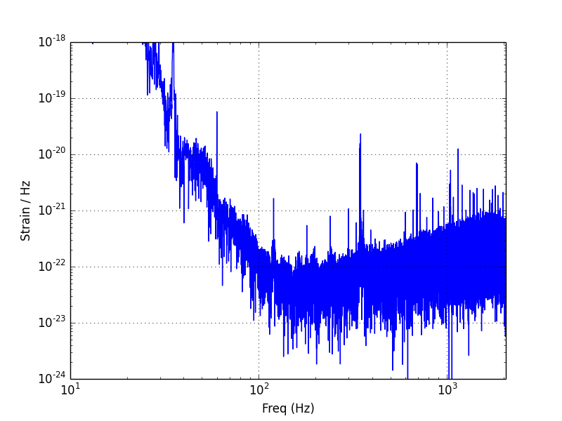
After using Welch's method:

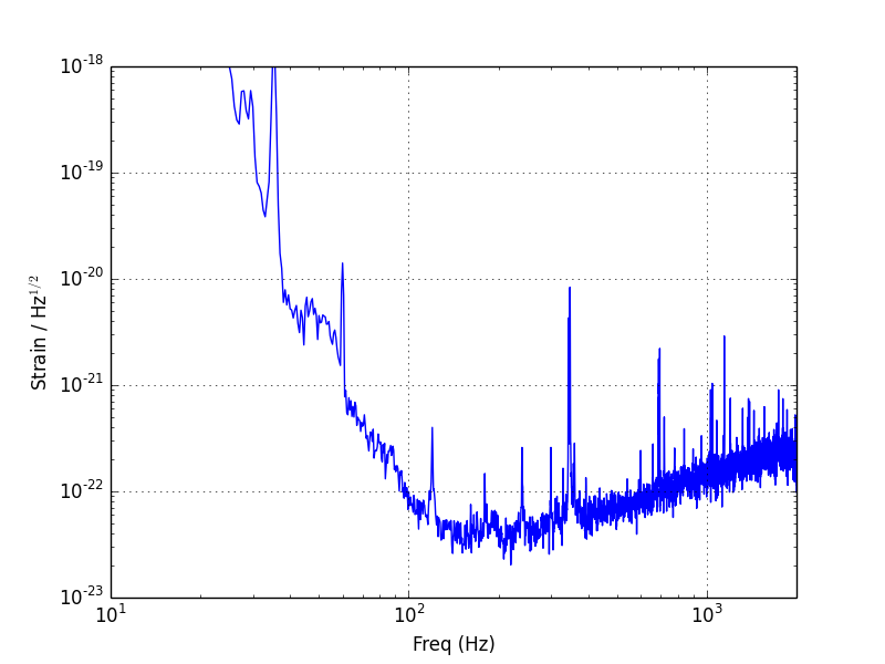
The example plots are from GWOSC.

Yi Qiu